第一章 算法简介
二分查找
下面是二分查找的实现代码,// 代表向下取整。
1 | def binary_search(list, item): |
大 O 表示法
为检查长度为 n 的列表,二分查找需要执行 log n 次操作,使用大 O 表示法,可以表示为 O(log n)。
大 O 表示法指出了平均情况下的运行时间。
常见的大 O 表示法
O(log n),也叫对数时间,如二分查找。
O(n),也叫线性时间,如简单查找。
O(n * log n),如快速排序。
O(n²),如选择排序。
O(n!),如旅行商问题。
启示
谈论算法的速度时,我们说的是随着输入的增加,其运行时间将以什么样的速度增加。
算法的运行时间用大 O 表示法表示。
第二章 选择排序
数组和链表
数组中的元素在内存中都是相连的,链表中的元素可存储在内存的任何地方。
比如六个人去看电影,数组就意味着六个一起的座位,链表相当于六个人分开坐。
链表的优势在插入元素方面,数组的优势在于随机读取元素。
| 数组 | 链表 | |
|---|---|---|
| 读取 | O(1) | O(n) |
| 插入 | O(n) | O(1) |
| 删除 | O(n) | O(1) |
选择排序
比如我想把自己听过的歌曲根据播放量从小到大排序,如果使用选择排序的话,就是先从全部的歌曲中找出播放量最少的写在纸上,然后找出第二少的再写到纸上,直到最后一个。
要找出播放量最少的歌曲,必须检查每一首歌,需要的时间是 O(n),对于这种时间为 O(n) 的操作,需要执行 n 次。所以需要的总时间为 O(n * n),即 O(n²)。
随着选择排序的进行,每一次需要检查的元素数在逐渐减少,到最后一次需要检查的元素只有一个,为什么运行时间还是 O(n n) 呢?这是因为从 n,n-1… 2,1,平均每次检查的元素数为 1/2 n,所以运行时间为 O(1/2 n n),大 O 表示法省略了常数。
下面是选择排序的实现代码
1 | def findSmallest_index(arr): |
第三章 递归
https://stackoverflow.com/questions/72209/recursion-or-iteration/72694#72694
Loops may achieve a performance gain for your program. Recursion may achieve a performance gain for your programmer. Choose which is more important in your situation!
第四章 快速排序
快速排序的原理:先从数组中选出一个基准值(pivot),然后找出比基准值大的元素和比基准值小的元素形成两个数组,然后合并成一个数组。
下面是快速排序的实现代码,进行了递归操作。
1 | def quicksort(arr): |
如果有 n 个元素,平均情况下可以分成 O(log n) 层,即栈长为 O(log n),每层的运行时间为 O(n),所以运行时间为 O(log n) O(n) = O(n log n)。
这一章的图画的挺好的
第五章 散列表
Python 提供的散列表实现为字典,可以使用 dict() 或者 {} 来创建散列表。
在访问 https://www.baidu.com/ 的时候,计算机将其转换为 IP 地址 180.76.76.76,这个过程被称为 DNS 解析,散列表是提供这种功能的方式之一。
散列表还可以用作网站的缓存:缓存是一种常见的加速方式,缓存的数据则存储在散列表中。
以下内容编程语言都实现好了
冲突
散列表可能出现冲突,处理冲突的办法有很多。
解决冲突最简单的办法:如果两个键映射到了同一个位置,就在这个位置存储一个链表。然而这就造成了性能的下降。
性能
良好的性能需要:较低的填装因子和良好的散列函数。
填装因子 = 散列表包含的元素数 / 位置总数,一旦填装因子超过0.7,就该调整散列表的长度。
散列函数最理想的情况就是将键均匀地映射到散列表的不同位置。
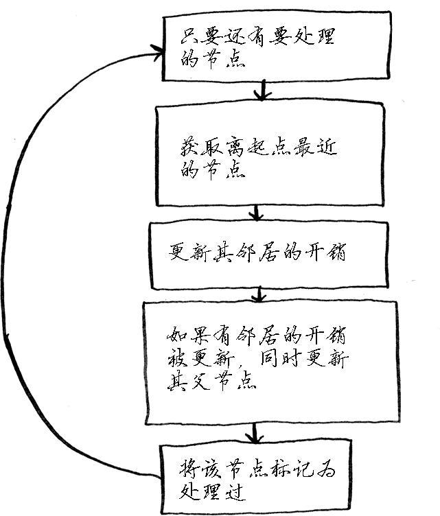
第六章 广度优先搜索
广度优先搜索(breadth-first search ,BFS)
相关的问题一般与队列有关,广度优先搜索一般能找出段数最少的路径。
下面是书中的一个实例,寻找名字中最后一个字母是 m 的人,一层一层朋友圈的寻找。
1 | from collections import deque |
第七章 狄克斯特拉算法
广度优先搜索用于在非加权图中查找最短路径。
狄克斯特拉算法用于在加权图中查找最短路径。
- 仅当权重为正时狄克斯特拉算法才管用。
实例
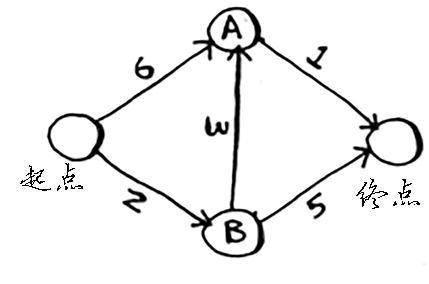
算法
过程
首先遍历起点的邻居
| 父节点 | 节点 | 开销 |
|---|---|---|
| 起点 | A | 6 |
| 起点 | B | 2 |
| 终点 | – |
因为 B 的开销最小,更新 B 的邻居
| 父节点 | 节点 | 开销 |
|---|---|---|
| B | A | 5 |
| 起点 | B | 2 |
| B | 终点 | 7 |
现在 A 的开销最小,更新 A 的邻居
| 父节点 | 节点 | 开销 |
|---|---|---|
| B | A | 5 |
| 起点 | B | 2 |
| A | 终点 | 6 |
更新完成
代码
1 | # the graph |
第八章 贪婪算法
典型的问题:教室调度问题。不再作详细记录。
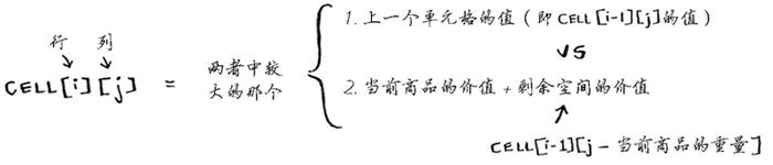
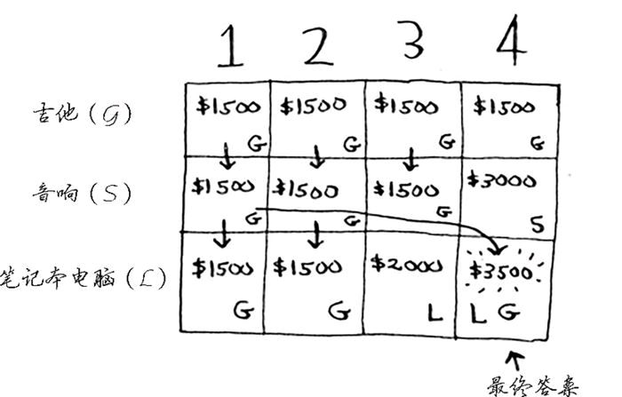
第九章 动态规划
每个动态规划问题都从一个网格开始,先解决子问题,在逐步解决大问题。这种问题就是找公式,画表格。
最典型的问题就是背包问题。
实例:背包最多装4斤东西,可选的东西有 3000 元的音响(4斤),2000 元的笔记本电脑(3斤),1500 元的吉他(1斤)。
这是计算公式。
这是根据公式画出的表格。
本书到此完结。